WSJT-X Wide Graph Optimization for EME use - Bob Atkins

WSJT-X Wide Graph (waterfall) optimization for EME use

The Wide Graph window in WSJT-X is a waterfall display of the signals present in the receiver audio output bandwidth. Since WSJT-X uses USB mode, this is typically from about 300Hz to 2500Hz, though some more recent, digital based receivers may offer a wider bandwidth option. For the purposes of this article I'll be talking about the audio output from the transceiver I use myself, The Yaesu FT-897. This is a conventional radio (not SDR) and as far as I know doesn't use digital processing in the audio output stages (unless digital based filtering is selected). I will also to focused on the use of the wide band display in connection with microwave EME, where signal spreading and widely spaced tones are found and QRM from other stations is rare.

Important note: When the flattening option of "flatten" is chosen, only the visual display of the spectrum is affected. The actual audio used by WSJT-X for decoding is NOT flattened. Neither are any saved .wav files. However, when the "reference spectrum" (Ref Spec) option is chosen, both the visual display data and the actual data used for decoding has flattening applied, as does any saved .wav files.

The waterfall display shows the audio spectrum as a function of time, with the amount of energy at any particular audio frequency represented as regions of different colors or intensity of colors. An example is shown below.

The wide graph display is used to locate WSJT-x digitally encoded signals and establish their "Base" frequency by identification of a pilot tone (for JT65), a lower frequency tone (for JT4) or other reference point (QRA64). It has no effect on the decoding of signals. If the right base frequency is chosen, the visibility of the trace on the Wide Graph is of no importance to decoding. In fact if both stations are GPS locked and exactly on frequency then you don't really need the wide graph at all! The one caveat is that the signal should be somewhere within the frequency range covered by the wide Graph

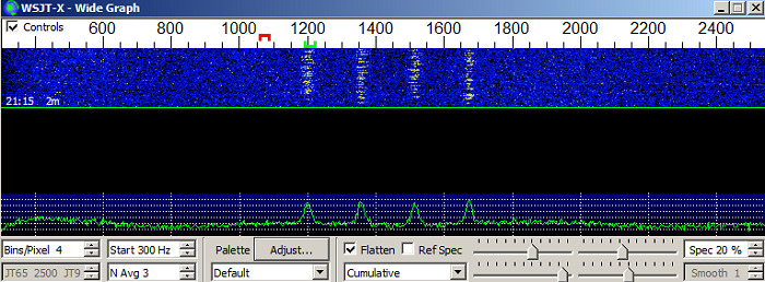
This is a JT4 signal on 10Ghz which decodes as 1757 -14 1.8 1201 $# G3WDG OK1KIR RRR. The base tone in this case is at 1200Hz.

Optimization

Since the user normally wants to be able to identify the signal and select the base frequency, it's obviously desirable to optimize the wide graph display for visual clarity. In the above example, with a reactively strong signal there's no problem, but if the signal is weak or spread even wider, identifying it can be harder. Here are a series of signals, decreasing in intensity by 5dB per step. As you can see, in the last step (top of the graph), it's very hard to distinguish the tones from the background.

There are three sets of parameters which can be adjusted to maximize the visibility of weak and/or spread signals. They are:

The color palette and the display gain and offset settings
The spectrum background flatness
The values for Bits/Pixes (the range of frequencies represented by each pixel of the display) and N Ave (the number of samples averaged before plotting)

I will cover each of these parameters in detail but here's the bottom line for maximizing the visibility of weak and widely spread signals. (1) Set a value of at least 4 for averaging 6 may be better) and a value of 3 or 4 (higher the better) for bits/pixel. (2) Do whatever you can to produce the flattest possible audio spectrum. (3) Optimize the display be choosing a good palette and tweaking the gain and zero sliders for maximum visibility of a weak signal.

Now the details and explanations:

(1) The color pallete and display settings

The display is made up of 9 colors, each representing a different signal strength. These 9 colors and their order is defined by the color palette chosen. WSJT-X has a number of choices, plus you can define your own, or import one.

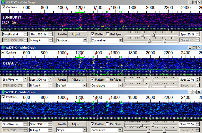
The first thing to know about color palettes is that there's is no "magic" palette which will outperform all others. You can make a very bad palette, where all the colors are the same or very similar, but if the colors are reasonably different and distinct, all palettes are pretty equally effective at showing weak or spread signals, provided you have gain and zero optimized for that pallete. Gain the the upper left slider and zero is the upper right slider. However I think there are some palletes that are slightly better than others, at least to my eyes. The default pallete is pretty good. I also like the "Scope" pallete and the "Sunburst" pallete. So the choice of pallete is up to you. Maybe start with the Default and then try a few others, re-optimizing gain and zero each time.

You can create a user defined pallete by selecting "user defined" and clicking on "adjust" then double right clicking on each color. you can also import and export palettes. They are stored in a text file with a .pal extension. The format is simply a list of 9 R;G;B color definitions, e.g.

0;0;0
255;255;0
255;0;127
0;255;0
255;85;0
85;170;0
0;0;255
85;170;255
255;255;255

The best way to do this is to find a really weak signal and tweak gain and zero for maximum visibility. A weak signal could be a "birdie" somewhere in the spectrum. These aren't normally hard to find! Alternatively you can use one of the sample files that come installed in WSJT-x. These are normally found in the directory C:/user//Appdata/Local/WSJT-X/save/samples/. You can load a file via the WSJT-X File - Open drop down menu. When load a file (which is an audio recording), it should appear on the Wide Graph plot. You can make the signals weaker by going to File - Settings - Advanced menu and entering a value in the "Degrade SNR of .wav file" field. The larger the value, the lower the SNR of the signal will be and the weaker the traces will appear.

When you are looking at weak signals you're only really looking at a transition between two levels, often the fist and second levels. So what's important in this context is good contest between the first two levels. Black/White, Black/Yellow, White/Black etc. The other colors only really come in on strong signals.

Again there is no "magic" setting that will give you the best visibility of weak traces with all palettes. In general I find that positing to the left of center of the zero slider work better for me. I set the zero slider to some value, then move the gain slider from left to right until different colored pixels just start to appear on the screen. I often find I'm setting the zero slider all the way to the left, then adjusting the gain so that a few pixels start to light on in the screen over the background color.

Background Flatness

Since you are looking for weak signals slightly above the background signal level, and those signals might spread out across a wide slice of the spectrum, maximum visibility of those signals will be achieved with a uniform low background. The signals may be a small fraction of a dB above the background, so it's important the the wide graph trace of the background be as uniform as possible. This is achieved by flattening the incoming audio spectrum and there are three ways to do this, which in order of complexity are:

Use the automatic "flatten" check box in the Wide Graph window
Preferred Option - Save a reference spectrum and use the "ref spec" check box in the Wide Graph window
Use external hardware or software to flatten the audio spectrum before it gets to WSJT-X

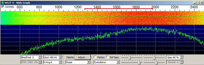
Most rigs no not produce an audio output that's flat across the spectrum. For example, here's what the audio from my FT-897 looks like with no flattening:

As you can see it peaks in rises to a peak at 1800-2000Hz then falls off. The waterfall display is multi colored and it would be be hard to see signals and impossile to see weak and/or spread signals. WSJT-X provides no dB scale for the variations in audio so you cant quantify anything from this display. At present (WSJT-X 2.3), this is the actual audio which is used for all processing (decoding) in WSJT-X

(1) Automatic Flatten Spectrum

- this is the simplest option. All you do is check the "flatten" check box and WSJT-X will attempt to flatten the audio spectrum in the best way it can. Depending on the original shape of the audio spectrum the result may be OK, good or very good. There's no way to make any adjustments, basically you get what you get and if it's not perfect, you live with it. For normal operation this option usually works well enough. However for the detection of really weak and widely spread signals, the flatter the spectrum the better. This does not affect the RAW audio used by WSJT-X for decoding.

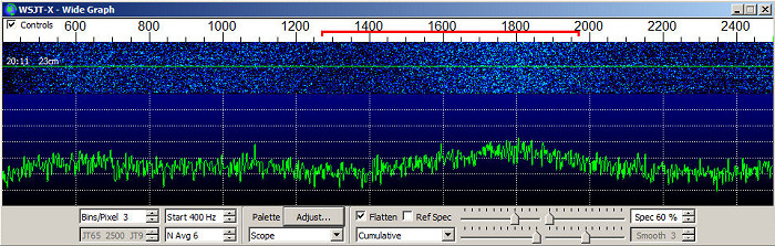
Here's what the automatically flattened spectrum from the FT-897 looks like:

This is obviously much better as you can tell from the much more uniform waterfall display. The spectrum still isn't totally flat as you can see from the lower plot. Just how flat it is you can't tell because WSJT-X provides no actual values on the X axis. It is clear though that the spectrum could be flatter and the waterfall display could be more uniform. NOTE that the actual audio used bt WSJT-X for decoding is NOT flattened in this case. The flattening is only applied to the Wide Graph display.

(2) Use a reference spectrum

- WSJT-X also gives you the option of saving a reference spectrum. This will usually give a better result than the automatic flattening option,so it's always worth trying. To use the reference spectrum option you point the antenna a quiet part of the sky so you have no birdies of other QRM signals visible on the waterfall or you can switch your preamp input to a 50ohm load if you can't find a QRM and birdie free signal. You then go to the "tools" menu option in WSJT-X and select the "measure reference spectrum" option. You wait for about 60 seconds while WSJT-X measures and averages the audio spectrum. The exact time you wait doesn't really matter. Then you click on the "STOP" button. At that point you will see a message box telling you that the reference spectrum has been saved. Now when you are looking at real signals, instead of checking the "Flatten" check box in the wide graph window, you check the "Ref Spec" button. This time WSJT-X will use the shape of the reference spectrum to help it figure out how to flatten the background of the incoming audio signal. The results may be better then the "automatic flatten" more - or they may not. Whichever method gives the flatter and more uniform background is the one to chose. Again you have no control over what WSJT-X does. You get what the program gives you and there are no adjustable parameters.

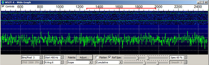
Here's the audio spectrum from the FT-897 after taking a 60 second reference spectrum and then checking the "Ref Spec" box. WSJT-x flattens the spectrum based on the data in the reference spectrum file and does a good job. This flattened audio is spectrum is the one which is actually used for decoding

This is much better. The waterfall display is now pretty uniform all the way across the display. In this case, this is probably all that is needed. There's not a lot (and probably not anything) to be gained by going to external spectrum flattening as described below. NOTE that in this case, WSJT-X used the flattened audio spectrum for decoding and analysis. Note here that you must be using the Rx with the same settings to receive the Signals displayed on the waterfall as were used when the reference spectrum was taken. For example, if you change the Rx passband width (as is possible on some rigs), you have to take a new reference spectrum. If your waterfall background doesn't look smooth and uniform, you might want to take a new reference spectrum, because something has probably changes.

NOTE: The bottom line here is that you should use the Reference Spectrum option for the best possible performance. The Flatten option is a "quick and dirty" solution that works most of the time but doesn't give the best results.

NOTE2: Added 12/19.20 - It is confirmed that, on version of WSJT-X at least up to 2.3.0, if you use the "flatten" option, all processing (decoding) is done on the RAW audio data, with no flattening applied. The flattening is only an aid to use of the visual Wide Graph. This can, in some cases, lead to missed decodes on weaker signals when using modes with a wide bandwidth (i.e. a bandwidth close to the audio bandwidth of the receiver). This would be most likely to happen on the higher microwave bands. If a reference spectrum is used, all processing is done on the flattened spectrum, leading to more reliable and better decoding performance when decoding weak signals. Again, the recommendation is to use the REFERENCE SPECTRUM option for microwave EME.

(3) Flatten the audio spectrum outside of WSJT-X

- This potentially give you the most control over spectrum flattening, though it may not be worth the effort since the the reference spectrum option works very well. Some advanced digitally based SDR receivers may already offer options to tailor the shape and width of the audio spectrum. If so then that's the way to do it. You can still check the "Flatten" check box if you wish. It seems to do some level shifting as well as flattening and the result may be better then not checking either the "Flatten" or "Ref Spec" boxes. Try it and see. If you don't have a super fancy digital receiver and are stuck with a fixed analog audio output ("you get what you get"), there are ways to tailor the audio spectrum. I use an FT-897, which provides "you get what we give you" audio output. The spectrum is far from flat and there are no built in tools to flatten it. So what do you do?

The "brute force" solution would be an external analog audio equalizer box with multiple frequency channels, each of which can be adjusted for gain. Fortunately there a much cheaper (free) and more elegant digital solution (if you are using a modern Windows operating system). It's called "Equalizer APO" and it's described as "Equalizer APO is a parametric / graphic equalizer for Windows. It is implemented as an Audio Processing Object (APO) for the system effect infrastructure introduced with Windows Vista". I'm no expert on "audio processing objects", but this application appears to sit between the audio input to the PC (which is my case is via the microphone input) and any software that tries to access that audio input. It can be downloaded from https://sourceforge.net/projects/equalizerapo/. Installation and use are fairly straightforward and there's a WIKI at https://sourceforge.net/p/equalizerapo/wiki/Documentation/. You can find more help on use at https://equalizerapo.com/

Just to repeat my earlier comment, the reference spectrum option usually does a very good job, so it additional flattening outside of WSJT-x is normally not necessary.

Bits/Pixes and N Ave

The visibility of weak traces and widely spread signals can be significantly enhanced by optimization of Bit/Pixes and N Ave. N Ave is the number of measurements averages before the data is plotted on the wide graph display. Each measurement seems to take about 1/2 second,so if you average 6 measurements the display will update (plot a new line) about every 3 seconds. Obviously this affects the speed at which the display scrolls gown the screen. I find a value of between 4 and 6 to be a good compromise between visibility and speed of scrolling. You want a line to be drawn for a weak signal and that line to have the best contrast with the background. I think an N Ave value between 4 and 6 does this best.

Bits/Pixel sets the horizontal axis of the wide graph plot. Each "bit" is the value of a small frequency segment of the audio spectrum. It's width depends on how WSJT is slicing up the FFT (Fast Fourier Transform) of the audio spectrum. I don't know the exact value but it's probably less than 1 Hz. A low value of Bits/Pixel "smears out" the data over a large area, while a higher value concentrates the data into a smaller region which makes it easier to see.

However, the Bits/Pixel setting does something else in additions, it controls the frequency range of the wide graph. If that range is larger than the bandwidth of the audio signal, WSJT-X gets upset when it tries to automatically flatten the audio spectrum, especially if the spectrum has a sharp cutoff. So you have to balance Bits/Pixel with the width of the Wide Graph. First make the wide graph display as small as possible by frequencies the width of that windows. There's a minimum width, which seems to be about 770 pixels, so set it to that. The range of frequencies covered by the plot is then determined by the settings of start frequency and bits/pixel. The values of these variables that will work depends on the width of your audio spectrum. You can try 400Hz for the start frequency and 3 or 4 for the Bits/pixel setting. You're basically looking for the lowest value of start (above about 200Hz) and the highest value of bits/pixel (probably 3 or 4) that will give you a uniform wide graph background. Again, that will depends on the width and flatness of your audio spectrum.

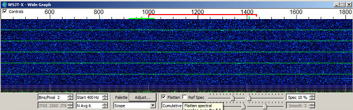
There's a signal here - can you see it? An experienced eye can probably see it, assuming the background is flat. If the background isn't flat it would be impossible to tell background fluctuation from a signal. Bits/Pixel is set to 2.

It's a QRA64C signal at somewhere around -20dB. There's no pilot tone in a QRA64 signal and in sub mode C the tones are spread out over about 440Hz. QRA64C would be used on 1296 MHz. For 10Ghz submode D would typically be use, with the tones spread out over about 880 Hz, making the signal even harder to see.

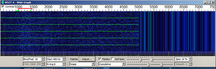
So what happens if we now change the value of Bits/pixel from 2 to 10? Well one thing is the range of frequencies shown is larger, large enough to extend outside the range of the audio signal from the rig, so this results:

It now becomes somewhat easier to see the QRA64C signal which is present between about 1000Hz and 1400Hz. It's still doesn't really stand out, but that's not surprising for a -20dB signal with tones dispersed over a 440 Hz range. But you can see it more clearly than when Bits/Pixel is set to 2.

A value of 10 for bits/pixel obviously results in a somewhat truncated display. With a normal bandwidth rig (2500Hz audio bandwidth) you can get a normal display with a value of 4 for bits/pixel and the wide graph windows resized to its minimum width. It will display something like 400Hz to 2550 Hz. With a rig having a 5kHz audio bandwidth you could bo to 8 bits/pixel and display 400 Hz to 4800Hz.

Weak signal example

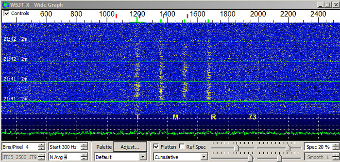
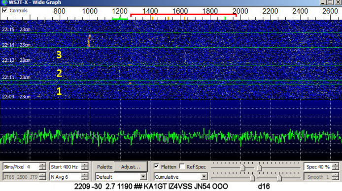
Finally, here's a weak signal trace (JT65C on 1296) that's visible on a well optimized wide graph display. In this case external audio flattening was used along with the "flatten" checkbox checked. Results using a reference spectrum with the "ref spec" box check would probably have been similar.

This signal decoded with the help of deep search at -30dB. I can't say that's an accurate number as there's always some uncertainty on weak decodes, but it's certainly pretty weak!. Period #1 decoded as "KA1GT IZ4VSS JN54 OOO" and the decode data was "d16" which indicated a deep search decode of a single frame with a confidence level of 6/10. The pilot tone is quite visible at 1200Hz, thought you can't really see the data tones. Period #2 shows the two tones (ca. 1200Hz and 1520Hz) for "RRR" reply to my "RO" transmission (which you can't see). Period #3 shows the two tones (ca. 1200Hz and 1630Hz) for "73", sent in reply to my "73" transmission (which again you can't see).

The 2d graph

I haven't really gone into much detail so far about the 2d graph which occupies the lower part of the Wide Graph display. Most of the time it's of lesser importance than the watefall display when using WSJT-X on the higher EME bands, but sometimes it can be quite useful. There are a number of display modes - Current, Cumulative, Linear Average and Reference. "Current" shows the spectrum obtained by the last FFT calculation over the period determined by the value of "N Ave". Cumulative shows the averaged spectrum over the current receive period since the start of the last minute (and so is an average of the "current" values. It's not 100% clear exactly what "Linear Average" is (though I think its probably an average of the power expressed in linear units rather than in dB), but it's the only mode which responds to the "smooth" parameter. "Reference" shows the last (current) reference spectrum.

The WSJT-x user guide suggests that "Linear Average" is good for signals subject to significant doppler spreading, an example of which would be JT4F mode on 10GHz. JT4F consists of 4 discrete tones spaced 157.5 Hz apart. At 10 Ghz each tone can be spread by as much as 200Hz, though an average value might be around 100Hz. The use of "Linear average" and "smoothing" can help to make those tones visible on the 2d plot. As with visual detection from the waterfall, a larger value of bits/pixel seems to help the identification of the tones.

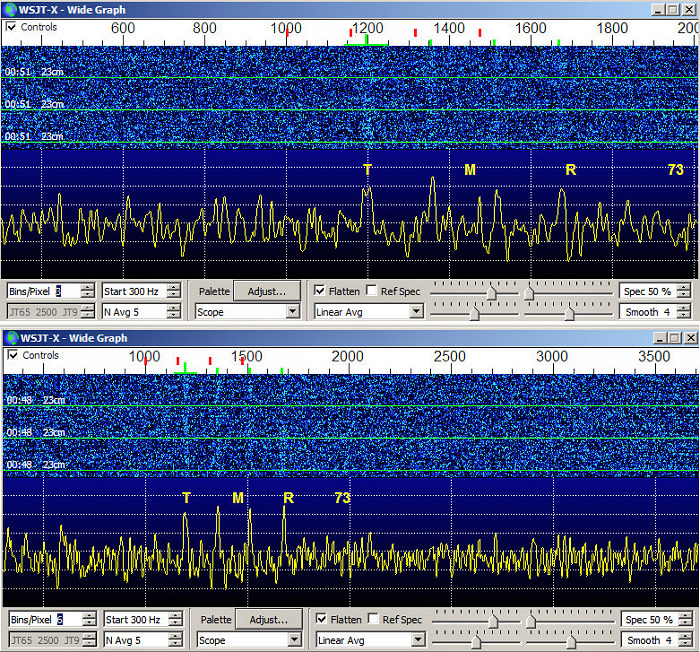
For example here are examples of a JT4F signal on 10Ghz at around -18dB with the display set to 3 bins/pixel and 6 bins/pixel, using linear averaging with a smoothing factor of 4. Spreading is reactively low (maybe ~ 70Hz).

The T, M, R and 73 labels on the 2d graph are where you would expect to see single tone (shorthand) messages appear. Just for the record "T" is the base frequency (nominally 1000Hz) and where a tuning tone appears if the DX station sends a tuning tone to establish the base frequency. "M" means I have received your tuning tone, please start sending the message. "R" is RRR, I have received your message, "73" is of course 73 and I have received you message and acknowledgment.

Acknowledgement

I'd like to thank Charlie, G3WDG, for his many helpful hints and suggestions and for initially encouraging me to start use WSJT-X! And of course Joe, WIJR and the whole WSJT-X development team for their work in developing WSJT-X.